Sometimes, time series data will have certain amount of inertia. This is when the values tend to stick around whatever value they currently are at. This is a slightly weird concept, so let’s generate some toy data that illustrates it.
import numpy as np
X = np.arange(0, 1, 0.001)

Y = [0]

for in it in range(1, 1000):
    Y.append(Y[i - 1] + np.random.normal(0, 0.05))
We have created two arrays. The first, X, which is just an evenly spaced range of 1000 points from 0 to 1. The second, Y, is defined iteratively, it starts and zero and then each consecutive value is the previous value plus a draw from a random normal with mean 0 and standard deviation 0.05.
When we plot Y against X it looks like this,
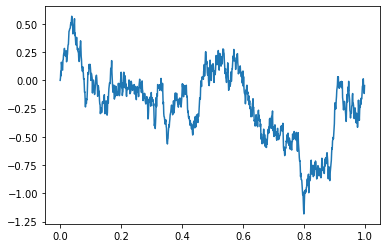
We can see, that rather than varying randomly around 0, this time series will wander occasionally to a certain level and then stay near there.
So, how do we model this kind of behaviour? With a lag feature. We can define a lag feature based on Y by
lagging_predictor = [0] + Y[:-1]For each index, this new feature will have the same value as the previous value of Y. We’ve also filled in the first value with 0.
Now let’s try some Linear Regression.
from sklearn.linear_model import LinearRegression
lagging_model = LinearRegression().fit(np.array(lagging_predictor).reshape(-1,1), Y)
When we look at the coefficients of this, we get an slope of 0.99 and an intercept of 0.003.
So our lagging model always predicts 0.003 plus 0.99 times the last value of Y. Which is a pretty good prediction! We can build more complex lagging features, but remember that linear combinations of features are taken care of by the fitting in ordinary least squares, so we don’t need to try those features ourselves.