It is common enough when looking at time series, to see a cyclic pattern. The values in our series will oscillate predictably. This may be driven by an underlying effect based on the time of day, or the day of the week, or even the day of the year. We can model this with a little feature engineering.
What we are talking about is a wave. Any wave can be modelled as a sine function. Suppose we have a time variable t that is normalised to have values between \(0\) and \(1\), then an arbitrary wave will be of the form
where
- A is the amplitude of the wave, that is, how high and low each crest and trough are
- f is the frequency, that is, how many times the wave repeats for a single unit of time
- o is the offset, how much the wave is shifted forwards
Now, these terms are quite non-linear, so they will by hard to model. However, we can do a little trigonometry. Thanks to the identity
we can rewrite the wave function as
We can then define \(B = A\sin(o)\) and \(C = A\cos(o)\), and then write any wave in the form
Now the only nonlinear term is the frequency of the oscillations.
Let's look at an example, suppose we have a time series that looks like,
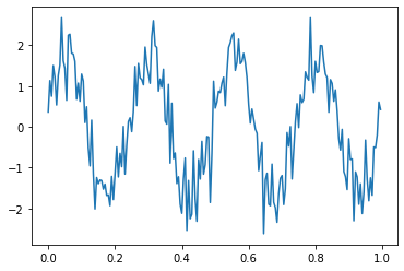
By eyeballing it, we can see a seasonal effect which repeats four times. So let's try some linear regression against the features \(\sin(x*4*2*\pi)\) and \(\cos(x*4*2*\pi)\).
import numpy as np
from sklearn.linear_model import LinearRegression
X, Y = # wherever our data comes from
sin_feature = np.sin(X*4*np.pi)
cos_feature = np.cos(X*4*np.pi)

harmonic_model = LinearRegression().fit([[s,c] for s,c in zip(sin_feature, cos_feature)], Y)
Now, I ran this regression myself, and the coefficents I got where, 1.69 and 0.38. So, we have
Which means our model's offset is
and our amplitude is
This is pretty good, as I generated the above data with an amplitude of 1.8 and an offset of 0.2 via
import numpy as np
X = np.arange(0, 1, 0.002)
Y = 1.8*np.sin(0.2 + X*4*2*np.pi)
We won't always have such an obvious cyclical pattern where we can spot the frequency by eye. We'll be looking at how to determine the appropriate frequency in these cases in a future post.